Spherical harmonics and Fourier series
During classical electrodynamics I had a bit of a hard time to understand what spherical harmonics are in a graphic way. If you have some intuition for Fourier series, I can give you a graphic way to understand the purpose of spherical harmonics.
Any square integrable function that is defined on a compact interval can be expanded into a Fourier series. That means that it can be written as a sum of various sine and cosine functions. If you just look at the $\cos(nx)$ and $\sin(nx)$ (where $n \in \mathbb N$) you see that they are higher frequencies or overtones.
You can also do this with functions of two dimensions. Say you have $f(x, y)$ defined on a square. Then you can express this as a Fourier series in $x$ and in $y$ by forming $\cos(nx) \cos(my)$, $\cos(nx) \sin(my)$ and so on. I have plotted the first few $\cos$ terms here:
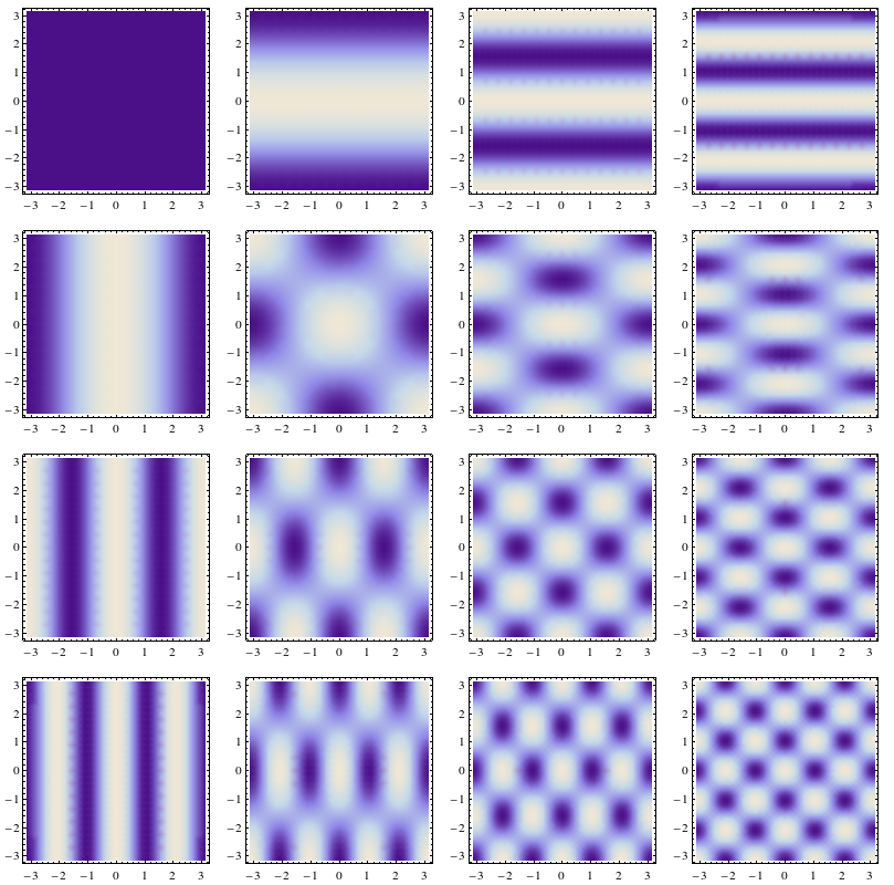
That was created in Mathematica 9 with:
GraphicsGrid[
  Table[DensityPlot[Cos[a x] Cos[b y], {x, -Pi, Pi}, {y, -Pi, Pi},
    PlotRange -> Full], {a, 0, 3}, {b, 0, 3}
  ]
]
These functions of $x$ and $y$ that are plotted above serve as a basis of the Hilbert space of square integrable functions $L^2$. You will need to include the terms with $\sin$ and the mixed ones as well.
You could also extend this and replace $\cos$ and $\sin$ with $\exp(\mathrm i x)$ and $\exp(- \mathrm i x)$ to get complex valued functions. The principle stays the same, except that you can now expand a complex function into such a series.
Spherical harmonics are the same idea, just on a sphere! Think of a function that is defined on a sphere, like the temperature on the surface of the earth. Then you can expand this temperature into a sort of Fourier series. The simple $\cos(nx)$ and $\sin(mx)$ now become the $Y_{l,m}(\theta, \phi)$ functions where $l$ and $m$ take the role of $n$ and $m$ before.
Since they are complex functions, one can plot the absolute value, the real or imaginary part. Here is the absolute value

That was generated with:
GraphicsGrid[
  Table[
    SphericalPlot3D[
      Abs[SphericalHarmonicY[l, m, theta, phi]],
      {theta, 0, Pi}, {phi, 0, 2 Pi}, PlotRange -> Full
    ], {l, 0, 3}, {m, -l, l}
  ]
]
The real part:

Generated with:
GraphicsGrid[
  Table[
    SphericalPlot3D[
      Re[SphericalHarmonicY[l, m, theta, phi]],
      {theta, 0, Pi}, {phi, 0, 2 Pi}, PlotRange -> Full
    ], {l, 0, 3}, {m, -l, l}
  ]
]
And the imaginary part last:

Generated with:
GraphicsGrid[
  Table[
    SphericalPlot3D[
      Im[SphericalHarmonicY[l, m, theta, phi]],
      {theta, 0, Pi}, {phi, 0, 2 Pi}, PlotRange -> Full
    ], {l, 0, 3}, {m, -l, l}
  ]
]