Reinforcement Learning with Frozen Lake
I have tried out reinforcement learning with the frozen lake example. In this post I will introduce the concept of Q-learning, the TensorFlow Agents library, the Frozen Lake game environment and how I put it all together.
When I play board games, I cannot stop myself from seeing the abstract rules, building a decision tree in my head and wondering how one could play an optimal round. This has led me to write a couple articles about board games. The one about Scythe features an implementation of parts of the game and the attempt to find a good game using just beam search. That was a first step, but I want to do better.
Reinforcement learning
Let us first take a look at this mental model that I have when playing a game. At any point it has a state $s$ and from there I can choose an action $a$ out of the set of actions $A$. If you play poker, the state $s$ would include your hand, the amount of money in the pot and which players are still in the game. The action set would include folding, calling or raising.
The player, an agent, finds themselves in a state $s \in S$ and needs to find an action $a \in A$ such that the final reward at the end of the game is maximized. This type of process is called Markov process. The problem of course is finding a policy that chooses the most promising action given the state. This policy is what differentiates a good player from a bad one.
But how do we find a good policy? This is the field of game theory. One way for instance would be to build the complete graph of states and actions and then see which paths always lead to a victory. For Tic-Tac-Toe there should be $9! = 361,880$ possibilities that the game could play out. A bunch are redundant due to the $D_4$ symmetry of the game, but even the full graph could be built up. If we know all possible further states in the game after taking a given action, we can find out whether we could always win it.
For any slightly more complicated game, the full graph cannot be constructed on a computer in a sensible fashion. Therefore one needs to have a less exact approach. We don't need to prove that we are going to win the game by taking a given action, it is sufficient to increase the likelihood of a high score or reward in the end.
Q-learning
This line of thinking leads us to Q-learning. The core is a function $Q$, which maps states and actions to the expected reward, so $$ Q \colon S \times A \to \mathbb R \,. $$ In other words, we can take the function $Q(s, a)$ and put in the current state $s$ of the game and an action $s$ that we are considering. The result will be the expected reward at the end of the game.
It is a crucially different to the greedy beam search that I have tried earlier. In the beam search, we just take the action that appears to be the best right now. In Scythe that might mean that you just play the “take money” action and get 2 victory points right there. In the long run, this will likely yield something rather mediocre, but it will appear to be the best thing at the moment. If one always takes the best option, one will switch between “take money” and “produce”, gaining 2 and 1 points in each round. After 20 rounds, one will have 30 points. That is not really great.
Q-learning instead factors in the expected total reward at the end of the game. This will allow us to invest some of the resources that we have into something that will turn out to yield more points a few rounds later.
Constructing the Q-function
Great, but how does one get this function? In an abstract way this function is just a table. It has all the states $S$ as rows and all the actions $A$ as columns. The cells contain the expected rewards. We just have to look up the row for the current state $s$ and can see the rewards for all actions $A$ directly.
This table would just be huge. For chess we have a number of states like $|S| = 10^{120}$ and around $|A| = 10^3$ possible moves. The whole Q-table would have $10^{123}$ entries. The amount of memory in a regular computer holds only around $10^{10}$ elements, so we don't have any chance of building an exact Q-table.
We need an approximation, some sort of effective model. And coming up with such functions needs some insights about the problems. One very versatile way to find effective functions is machine learning, deep learning in particular. There one specifies a model with a certain capacity and internal structure, feeds it a bunch of inputs ($s$ and $a$) and compares the output (rewards) of the model with the ones that actually came out. This works for classifying hand-written digits, extracting the sentiment of movie reviews and it also works for playing games.
Learning mechanism
How do we know what the reward per step should be? We just play the game with random actions, see what the end result is and distribute the reward onto the steps. The last step will get attributed the full reward. The second last step will have it diminished by a factor $\gamma \sim 0.95$. The third last step will see it diminished by $\gamma^2$ and so on. This way the lasts steps in the game will get a lot of weight, whereas the first steps will not really get a strong signal.
We can make this intuitive. When we play a game without knowing the game rules, we are just messing around. If we win the game, the last steps were likely having a good effect, whereas the first steps could have been awful and compensated by later actions. We don't want to give the first steps too much credit, at least not in the beginning of training. We can determine the Q-function really good at the end. When we are playing Tic-Tac-Toe and are at a really advantageous state $s_t$, perform the action $a_t$ and win the game, we know that $a_t$ was a really good idea, given that we already made it to $s_t$. We therefore want to give a strong signal to reinforce this behavior. The next time the simulation ends up at $s_t$, it will be certain that taking $a_t$ will give a good reward. Once that and other final steps are locked in, the agent can start to learn the second last step of the game. Given a state $s_{t-1}$ it can look at the actions $a_{t-1}$ that will bring it into the state $s_t$. The Q-function already has enough data to know which $s_t$ are a stepping stone to victory, so learning which $a_{t-1}$ to choose is pretty much determined by the knowledge that it already has. In this fashion it will learn from the late-game to the mid-game and then early-game.
Deep learning now comes in to give the Q-function some concrete form. It will be a network where there the input is a tensor that encodes the state $s$. The output will be a vector that contains the expected return for each action $a \in A$. We can have arbitrary layers in between to give the model enough capacity to learn.
The loss function is the sum of squared differences between predicted and actual rewards. We let the agent play the game until it has ended, compute the rewards for each step, and then train the agent on every single time step to make it learn the rewards for every action and step.
TensorFlow Agents library
These bits are already packaged in the TensorFlow Agents library. One has agents, environments, policies, states, actions and a training loop.
- The environment encapsulates the game or task at hand. It will take an action and return a new time step. This contains the current state of the game, the reward, the discount $\gamma$, information whether it is a start, mid or end step.
- The agent will work in the environment, observe the state and derive an action according to its policy. It has some internal state which is going to be trained with reinforcement learning.
- The policy is a mapping from states to actions.
There is a simple tutorial for DQN learning which I took as a starting point. It uses the Cart-Pole environment, but one can also try other ones.
The main idea in learning with deep Q networks is that one takes a deep neural network to model the Q-function.
Frozen Lake
I initially wanted to train an agent on Scythe, but that has the problem that the game state is really complex, and that there are many actions. Not all actions can be taken in each step, and some actions have details (like where to move pieces) whereas other have not (take money). So I thought that I should rather go and do something simpler and tried to do 2048. There the game state is finite, and there are always four actions that one could take. I have tried a bit, but it didn't really learn anything. There could have been a bunch of issues, so I eventually went for an even easier problem.
Introducing Frozen Lake, a really simple problem for the agent to solve. The authors describe it as this:
Winter is here. You and your friends were tossing around a frisbee at the park when you made a wild throw that left the frisbee out in the middle of the lake. The water is mostly frozen, but there are a few holes where the ice has melted. If you step into one of those holes, you'll fall into the freezing water. At this time, there's an international frisbee shortage, so it's absolutely imperative that you navigate across the lake and retrieve the disc. However, the ice is slippery, so you won't always move in the direction you intend.
In the simplest incarnation, there is a lake with 4×4 tiles
SFFF
FHFH
FFFH
HFFG
These symbols mean the following:
| Symbol | Meaning |
|---|---|
| S | Starting point, safe |
| F | Frozen surface, safe |
| H | Hole, fall to your doom |
| G | Goal, where the frisbee is located |
In the source code we can find a mapping from direction to numbers:
| Direction | Number |
|---|---|
| Left | 0 |
| Down | 1 |
| Right | 2 |
| Up | 3 |
Step table
With this we can build a table and write down where the movements will take us. This can be thought of a precursor to the Q-table.
| Index | Content | Left | Down | Right | Up |
|---|---|---|---|---|---|
| 1 | Start | Nothing | Frozen | Frozen | Nothing |
| 2 | Frozen | Start | Hole | Frozen | Nothing |
| 3 | Frozen | Frozen | Frozen | Frozen | Nothing |
| 4 | Frozen | Frozen | Hole | Nothing | Nothing |
| 5 | Frozen | Nothing | Frozen | Hole | Start |
| 6 | Hole | — | — | — | — |
| 7 | Frozen | Hole | Frozen | Hole | Frozen |
| 8 | Hole | — | — | — | — |
| 9 | Frozen | Nothing | Hole | Frozen | Frozen |
| 10 | Frozen | Frozen | Frozen | Frozen | Hole |
| 11 | Frozen | Frozen | Frozen | Frozen | Frozen |
| 12 | Hole | — | — | — | — |
| 13 | Hole | — | — | — | — |
| 14 | Frozen | Hole | Nothing | Frozen | Frozen |
| 15 | Frozen | Frozen | Nothing | Goal | Frozen |
| 16 | Goal | — | — | — | — |
We can even take this one step further and think of the most sensible actions in each tile. We want to take a short path directly to the goal. When we take away the holes, we can see the paths more clearly:
SFFF
F.F.
FFF.
.FFG
The last F in the top row is useless for us, we don't need that, it is a dead end. So let us remove that as well. I have added the same tiles with numbers such that our discussion becomes a bit easier.
SFF.   01 02 03 ..
F.F.   05 .. 07 ..
FFF.   09 10 11 ..
.FFG   .. 14 15 16
It is clear that if we are at the bottom-right F, we clearly must go to the right. All other options don't make any sense. So I can already mark the Right action for tile 15 as the most sensible one. How do we get to tile 15? Either we are at tile 14 and go right, or we are at tile 11 and go down. How do we get to tile 14? Most sensibly going down from 10. And to 11 we can get either by going down from 7 or right from 10. The others go the same way. I have also included 4 in the table, there the only sensible option is to go left. The following table therefore contains the most sensible options, and we would expect that the agent would learn exactly that.
| Index | Content | Left | Down | Right | Up |
|---|---|---|---|---|---|
| 1 | Start | Nothing | Frozen | Frozen | Nothing |
| 2 | Frozen | Start | Hole | Frozen | Nothing |
| 3 | Frozen | Frozen | Frozen | Frozen | Nothing |
| 4 | Frozen | Frozen | Hole | Nothing | Nothing |
| 5 | Frozen | Nothing | Frozen | Hole | Start |
| 6 | Hole | — | — | — | — |
| 7 | Frozen | Hole | Frozen | Hole | Frozen |
| 8 | Hole | — | — | — | — |
| 9 | Frozen | Nothing | Hole | Frozen | Frozen |
| 10 | Frozen | Frozen | Frozen | Frozen | Hole |
| 11 | Frozen | Frozen | Frozen | Frozen | Frozen |
| 12 | Hole | — | — | — | — |
| 13 | Hole | — | — | — | — |
| 14 | Frozen | Hole | Nothing | Frozen | Frozen |
| 15 | Frozen | Frozen | Nothing | Goal | Frozen |
| 16 | Goal | — | — | — | — |
Implementation
My final implementation is on GitHub. I will show the most important pieces here and explain what they do.
Environment
First we need to have the environment. This is where the agent will act upon. We can just load it from a “gym” and repackage that pure Python environment as a TensorFlow environment. This will convert the NumPy arrays into TensorFlow tensors.
def make_env():
    env_name = "FrozenLake-v0"
    train_py_env = suite_gym.load(env_name)
    train_env = tf_py_environment.TFPyEnvironment(train_py_env)
    return train_env
We can take a look at train_env.observation_spec(), that gives us the shape of the observation. In this case it is a just a single integer from 0 to 15, encoding the position of the player on the frozen lake. train_env.action_spec() gives us the shape of the action, and they are just a single integer from 0 to 3, encoding the direction as stated in the table above. With that information we can then construct a neural network.
Network and agent
We know that the network takes a state integer from 0 to 15 and it has to emit the Q-value for each of the four actions that can be taken. Putting such integers into a network doesn't work in any sensible way, they need to be encoded as vectors. The most trivial way to encode such an integer would be the one-hot encoding where one takes vectors of length 16 that look like this: $$ s_0 = (1, 0, 0, \ldots) \,,\quad s_1 = (0, 1, 0, \ldots) \,,\quad s_2 = (0, 0, 1, \ldots) \,,\quad \ldots $$
When we do that and multiply with a dense layer, each one-hot vector will pick out one of the columns of the matrix. We can therefore combine the one-hot encoding and the first dense layer into an Keras embedding layer which has 16 inputs.
In this simple problem we know that the Q-table can be constructed explicitly with a 16×4 table. Choosing the hidden size of the embedding layer as 4 directly gives us a single layer with the Q-table and also the correct output size.
We then also need to have an optimizer, a step counter and the compiled network to create the DQN agent. The loss function is taking the sum of the squared difference between predicted and actual rewards.
def make_tf_agent(train_env):
    dense_layers = [
        tf.keras.layers.Embedding(16, 4),
    ]
    q_net = sequential.Sequential(dense_layers)
    learning_rate = 1e-3
    optimizer = tf.keras.optimizers.Adam(learning_rate=learning_rate)
    train_step_counter = tf.Variable(0)
    tf_agent = dqn_agent.DqnAgent(
        train_env.time_step_spec(),
        train_env.action_spec(),
        q_network=q_net,
        optimizer=optimizer,
        td_errors_loss_fn=common.element_wise_squared_loss,
        train_step_counter=train_step_counter,
    )
    tf_agent.initialize()
    summarize_network(q_net)
    tf_agent.train = common.function(tf_agent.train)
    tf_agent.train_step_counter.assign(0)
    return tf_agent
Replay buffer
The training process needs some place to store the plays of the game. The agent will play the game in a first phase, and then it will be trained on that experience. This is the feedback mechanism which will make the agent play better next time. We give it some capacity, but there is not much special about it here.
def make_replay_buffer(tf_agent, train_env):
    replay_buffer_capacity = 100000
    replay_buffer = tf_uniform_replay_buffer.TFUniformReplayBuffer(
        data_spec=tf_agent.collect_data_spec,
        batch_size=train_env.batch_size,
        max_length=replay_buffer_capacity,
    )
    return replay_buffer
Collecting episodes
The collection of episodes is pretty much as described in the theory of Q-learning. The agent will start with a fresh environment. Then it will take a look at the current state and derive an action using the policy. It will tell the environment about the action and the former will perform the latter and it will result in a new state. This transition is put into the replay buffer. Once the episode has finished, the environment will automatically start anew.
def collect_episode(env, policy, num_episodes, replay_buffer):
    episode_counter = 0
    env.reset()

    while episode_counter < num_episodes:
        time_step = env.current_time_step()
        action_step = policy.action(time_step)
        next_time_step = env.step(action_step.action)
        traj = trajectory.from_transition(time_step, action_step, next_time_step)

        replay_buffer.add_batch(traj)

        if traj.is_boundary():
            episode_counter += 1
Evaluation metric
We have the loss function, but that doesn't tell us so much. We also need to have a metric in order to evaluate our problem. We can take the average return over say 10 episodes. As the return is either 0 (fell into a hole) or 1 (made it to the goal), the average return will also be the average number of successes. Ideally we get it to 1.0. There is a slight catch to that because of a source of randomness. In the description of the problem, there was this last sentence:
However, the ice is slippery, so you won't always move in the direction you intend.
So the environment might not abide by the choice of action and do something else, but never goes into the opposite direction. This means that the agent has to cope with random failures, and therefore the average return cannot be exactly 1.0 but only get close to it.
Main loop
We can now put everything together into a main loop. I have added a little bookkeeping for the weights, loss and metric, they are plotted every 50 iterations of the training such that we can track progress.
def main():
    train_env = make_env()
    tf_agent = make_tf_agent(train_env)
    replay_buffer = make_replay_buffer(tf_agent, train_env)
    collect_episodes_per_iteration = 1
    batch_size = 64
    dataset = replay_buffer.as_dataset(
        num_parallel_calls=3, sample_batch_size=batch_size, num_steps=2
    ).prefetch(3)
    iterator = iter(dataset)
    collect_episode(
        train_env,
        tf_agent.collect_policy,
        collect_episodes_per_iteration + batch_size,
        replay_buffer,
    )

    returns = []
    losses = []
    weights = []
    num_iterations = 20000
    eval_interval = 50
    num_eval_episodes = 10
    for _ in tqdm.tqdm(range(num_iterations)):
        collect_episode(
            train_env,
            tf_agent.collect_policy,
            collect_episodes_per_iteration,
            replay_buffer,
        )
        experience, unused_info = next(iterator)
        experience2 = trajectory.Trajectory(
            experience.step_type,
            experience.observation,
            experience.action,
            experience.policy_info,
            experience.next_step_type,
            experience.reward,
            experience.discount * 0.95,
        )
        losses.append(tf_agent.train(experience2).loss)
        step = tf_agent.train_step_counter.numpy()

        if step % eval_interval == 0:
            avg_return = compute_avg_return(
                train_env, tf_agent.policy, num_eval_episodes
            )
            returns.append(avg_return)
            weights.append(tf_agent._q_network.layers[0].get_weights())
            plot_returns(eval_interval, returns)
            plot_loss(losses)
            plot_weights(eval_interval, weights)
Results
With all that in place, I was able to start training. It took a little bit to get all the tensor shapes sorted out, understand how the things have to be combined and so on. Eventually it started doing things. In the beginning it wasn't able to finish the game, which seems intuitive. The network weights are initialized with random values, so the policy will generate random actions. Doing a random walk on a frozen lake will end in a hole rather soon, so there never was any return. By chance it eventually made it to the end. The number of successes started to go up.
But then the number of successes went down again. Eventually the agent seemed to have forgotten how to get to the goal. It was frustrating and I couldn't make any sense of it. Looking at the evolution of the 64 weights showed that virtually all of them were going up in about the same rate. The agent was learning that there are rewards, but no direction was special. This didn't make much sense. As a consequence the policy would become random again, as the rewards in all directions was the same.
Discount adjustment
One crucial thing was the adjustment of the discount. A coworker has pointed me to it. For some reason the environment has set it to 1.0. This means that once the agent finishes at the goal, all the steps that lead to it get a reward of 1. This means that it will reinforce all the steps that it has taken up to that point. We have no idea whether it went from start to finish in a straight line or did a lot of useless steps. It could have wandered a couple of laps around the middle hole before finishing. All these things would become encouraged. If enough silly movements become encouraged, it would fail to reach the goal quickly.
By setting the discount to 0.95, the reward will become concentrated on the last steps that the agent did. It will also encourage taking a short path from start to finish. With that in place, the whole training become much more focused and stable.
Average returns
The most clear data is in the average returns. We can see that over the training steps it goes up, and it consistently stays up. With just 10 episode in evaluation we don't get a lot of precision, but it still looks decent.
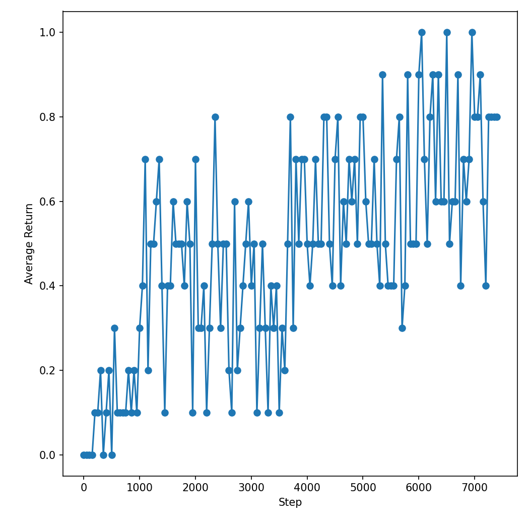
We would have to estimate the success rate of perfectly played games and take into account the effects of slippery ice. I think that there was a 10 % chance of slipping on every step, we do like 6 steps and not every slipping goes into a hole. So reaching around 80 % sounds pretty decent.
Loss
Looking at the loss confused me and my coworker quite a bit. What does that even mean? And why isn't it going down?
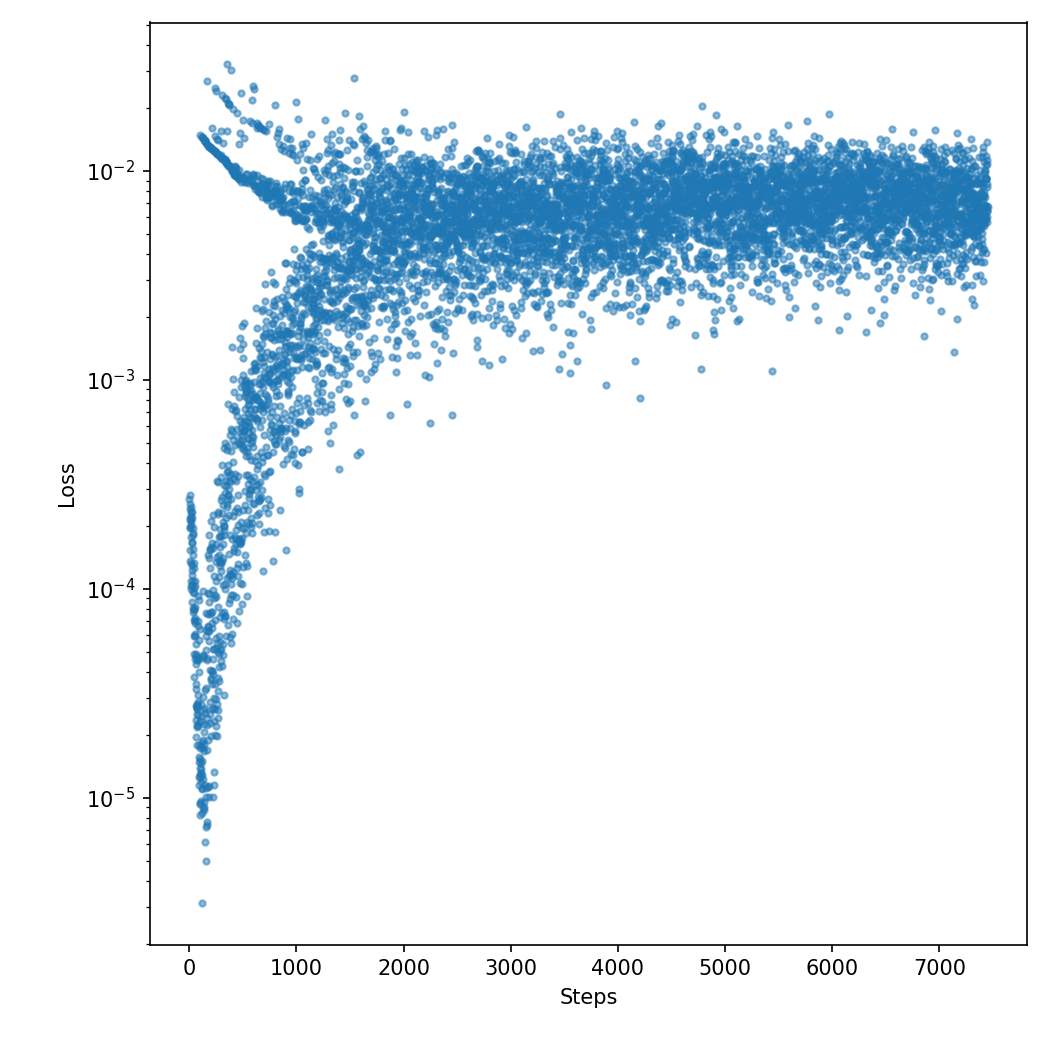
The answer can be found in the initialization. It is initialized with rather small numbers, so the predicted reward is around 0 for all states and actions. In the beginning the agent never finishes the game, so the actual reward is zero. That matches pretty closely, and the network is actually pushed towards having all weights at zero. This is the steep downward trend in the lower left part of the diagram.
But eventually the agent will finish. The loss will be large as the reward is 1, but the prediction was zero. This yields those outliers in the top left of the chart. Eventually the number of successes drives the weights towards more realistic values. The batches where all episodes end with failures and a reward of 0 meets a more optimistic prediction will yield larger and larger losses. This is the upward trend in the lower left part.
Eventually most batches will contain successes, so the two extremes of the losses start to meet. The whole cloud likely slowly goes down, but the trend is not visible because I forgot to include a smoothing curve in the plot.
Weights
There are 64 weights, and looking at all of them at the same times isn't so helpful. So let us take a look at the weights 14 and 15, the ones in the middle of the bottom row of the lake. I reproduce the two rows of the neighbor table from above as well.
| Index | Content | Left | Down | Right | Up |
|---|---|---|---|---|---|
| 14 | Frozen | Hole | Nothing | Frozen | Frozen |
| 15 | Frozen | Frozen | Nothing | Goal | Frozen |
The weight plot directly corresponds to the above table. The two rows are the two tiles, 14 and 15. The four columns are the four directions; left, down, right, up.
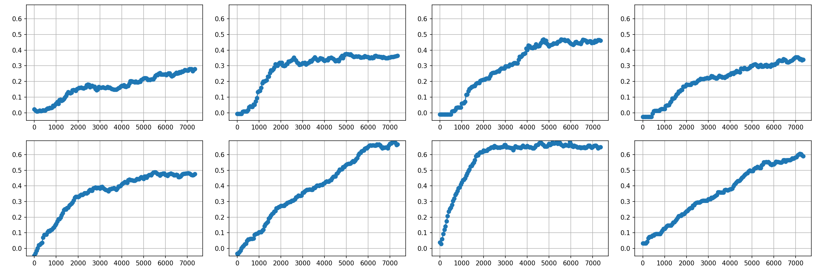
We can see that the steepest learning has happened on tile 15 into the right direction. That is satisfactory because we know that this will directly lead us to the goal. The weight above that, corresponding to tile 14 and the right direction, has also the highest value. Its learning is not as steep as for tile 15, because it had to learn the strategy for tile 15 first. Also there is another discount factor $\gamma$ in play such that the reward is a bit lower.
The curious thing is that for tile 15 the down direction is also rather large. This likely comes because going down doesn't do anything there. I am not sure whether it could slip there or it is a no-op. All it does it incur another discount factor $\gamma$, but it doesn't really hurt. So going down first doesn't hurt, it will still get the reward in the end.
Also strange is that for tile 14 going left ends in a hole. Yet the expected reward there is quite large. I don't quite understand why that is the case, perhaps the slippery ice has saved it enough times to learn that this is not a catastrophic action. Still going right is better.
We can compare this to the weights of the first rows. Here the expectation table looks like this:
| Index | Content | Left | Down | Right | Up |
|---|---|---|---|---|---|
| 1 | Start | Nothing | Frozen | Frozen | Nothing |
| 2 | Frozen | Start | Hole | Frozen | Nothing |
| 3 | Frozen | Frozen | Frozen | Frozen | Nothing |
| 4 | Frozen | Frozen | Hole | Nothing | Nothing |
I don't really see that the agent has learned so much here. The weights are still going up, so perhaps it would improve further. Due to the discount, the rewards there would be just around 0.8. This should still be enough for the network to learn. Perhaps we just need many more steps until it has learned the frozen lake topology properly.
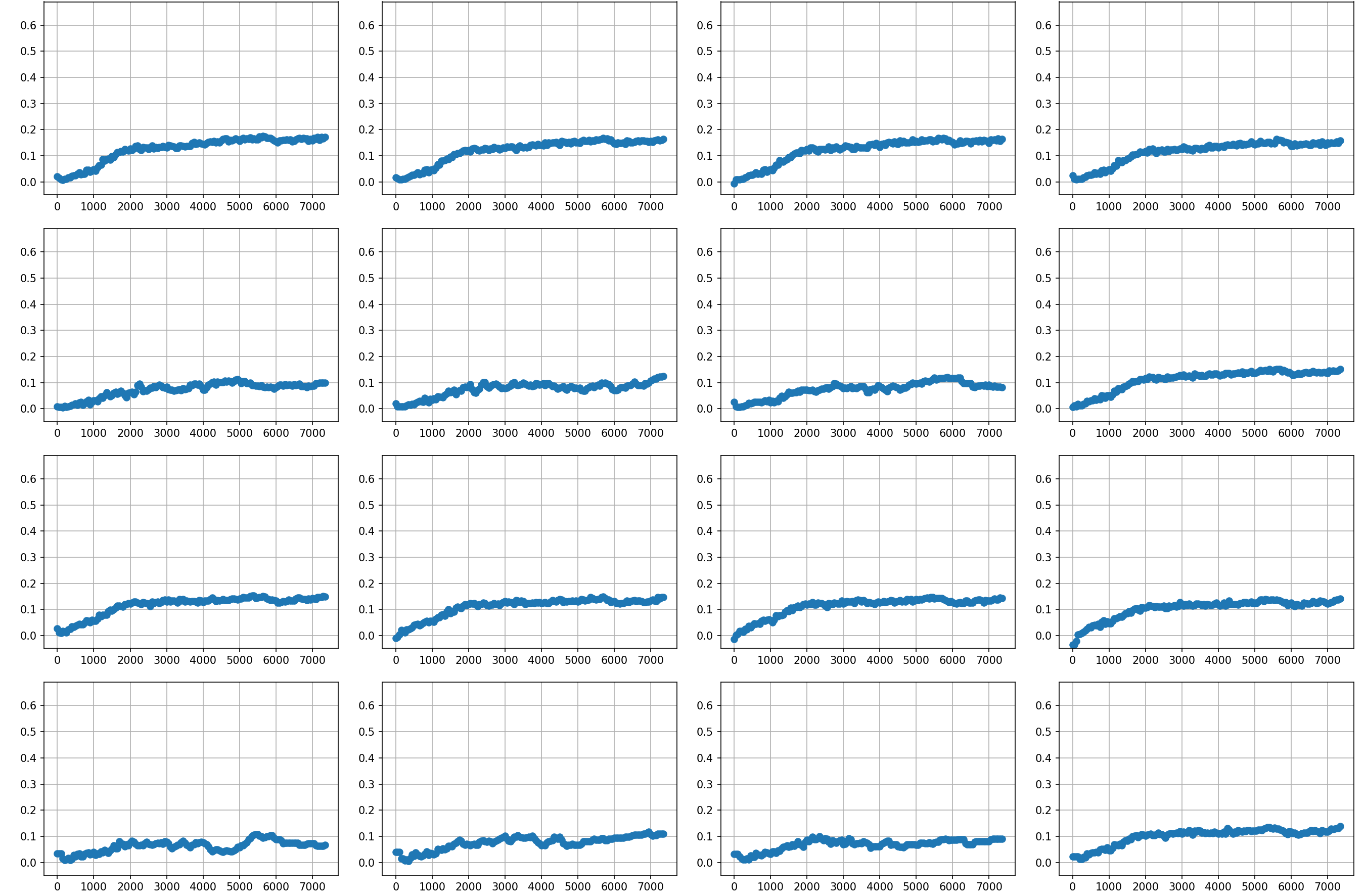
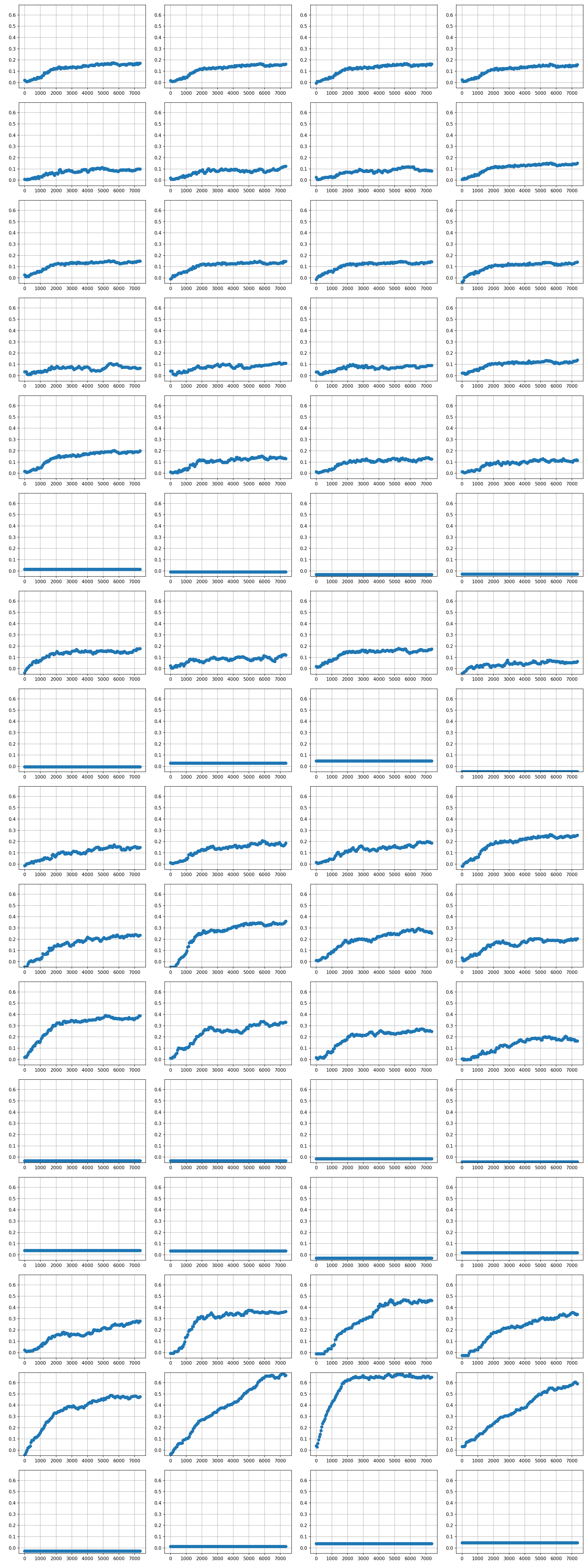
You can also have a look at the full plot weights. I unfortunately forgot the labels, but the structure is the same as the table. The ones with flat lines are the holes, there is no training feedback there because the agent never did a step away from a hole. Click on the image to enlarge it.
Conclusions
This has been a longer running project, I just put in a few days over a couple months so far. There were a few starting issues, but I think that I have solved them now. In order to get better results, I would need to play around with the batch size, the learning rate and the discount factor. Perhaps there are much better ways to tune those hyperparameters.
This simple game turned out to take quite a while to train on a CPU. There are so many steps needed for the average return to become somewhat sensible and there are just 64 parameters in the network that have to be learned. For more complicated games I will need larger networks and then it will take much longer to have enough training material for all these parameters.
I will have to see how I continue. The procedure will work for any game which has finite state and finite actions. Perhaps I will go and continue with 2048, but I also have the coin traiding in Nidavellir in mind.