Coin Upgrades in Nidavellir
Yesterday I've played Nidavellir, a game where one drafts a dwarf army to fight a dragon and seize the treasure it guards. It is just about the drafting, no actual fighting. The player with the best dwarf amy wins, and that is scored by points. Dwarfs are recruited in taverns, and one the players have to bid on the three taverns, and the players can then choose the dwarfs in order of highest bids.
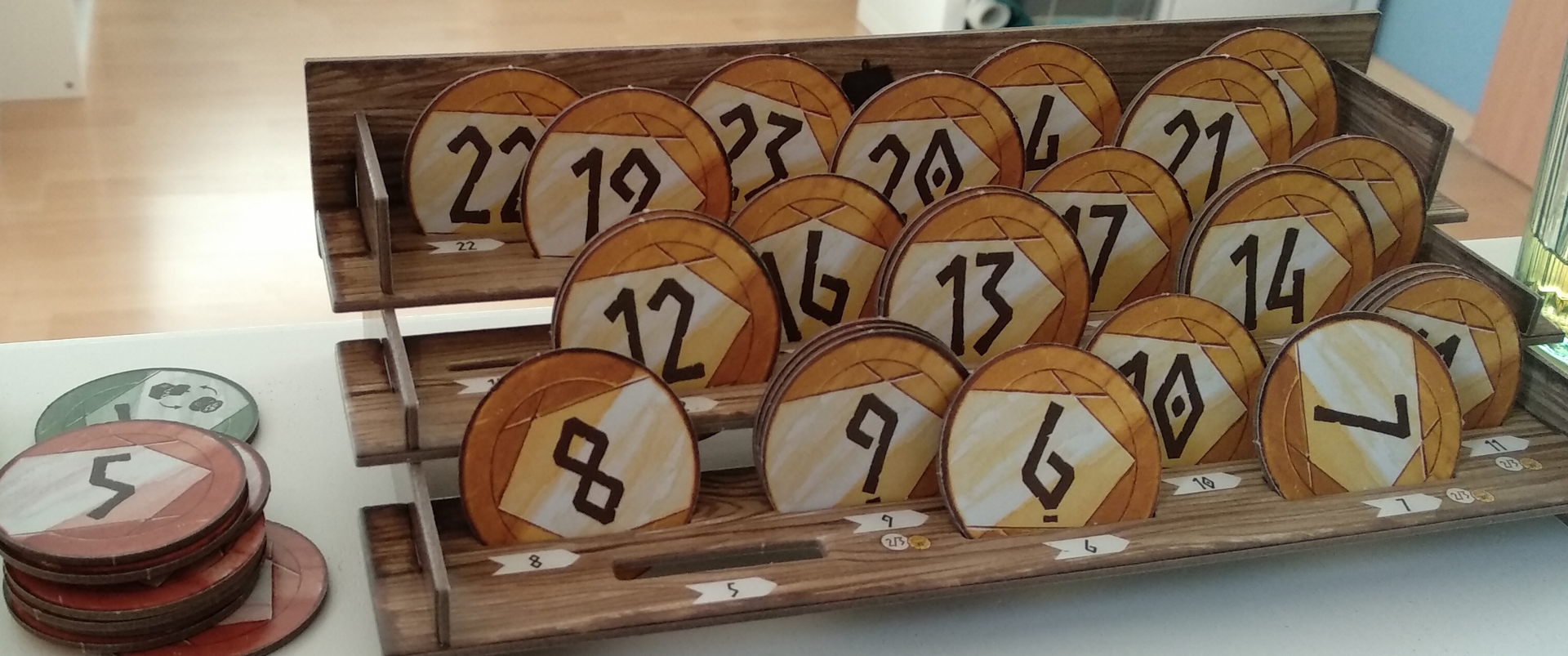
There is a side mechanism in the game for upgrading the coins. One always start with the coins valued 0, 2, 3, 4 and 5. One can bet with a special 0 valued coin in one of the taverns and reserve two coins for upgrading. From the two coins set aside, the higher one is upgraded by the value of the lower one. If one sets away coins 3 and 5, one the 5 will get replaced with 8. If there is no such coin left in the bank, one will get the next higher coin. There are three replicas from 5 to 11, two replicas from 12 to 14, and one replica from 15 to 25; at least when played with three players.
While I played the game for the first time, I was pretty distracted by figuring out the best coin upgrade strategy. The sum of all coins will contribute to the final score. Therefore it makes sense to upgrade them. And also they help in bidding.
Brute force
This is a problem where in each step there are $\binom 42 = 6$ possible ways to set away two coins. And there are only eight rounds, so in total there are just $6^8 = 1\,679\,616$ possible ways to play this. That is feasable with brute force and exploring the full graph. Some upgrades are not doable as the highest coin is just 25. Therefore the actual number of nodes in each level of the graph are these:
- 1
- 6
- 36
- 216
- 1,296
- 7,746
- 44,552
- 233,251
- 1,104,806
This is implemented as part of my game-simulation-sandbox. My Python implementation does around 10000 steps per second, so that is a decent pace. I have found the winning strategy yielding a sum of 58 to be these steps:
- 2, 3, 4, 5
- 2, 3, 5, 7
- 2, 5, 5, 7
- 2, 5, 7, 10
- 2, 7, 7, 10
- 2, 7, 10, 14
- 2, 7, 10, 24
- 2, 7, 17, 24
- 2, 7, 24, 25
One can see that all coins get upgraded. The 2 cannot be upgraded as it is always the smallest coin. And then it cleverly uses that the bank doesn't have the coins, so from 7 + 17 we don't get another 24 but the 25.
One can take a look at all the possible outcomes. This gives a distribution like this:

There are very few final states with cores higher than 50. And there is only one state with 58. This means that a search algorithm has to really work hard to find that optimal one.
Greedy beam search
As this problem can be done with brute force, we can evaluate other algorithms that only do a partial graph search. As I've used a greedy beam search in the last post about Scythe, I will try the same thing here.
Limiting this to the top 100 beams in every step, we only get a best strategy with a sum of 55:
- 2, 3, 4, 5
- 2, 3, 5, 7
- 2, 3, 5, 12
- 2, 5, 5, 12
- 2, 5, 10, 12
- 2, 5, 10, 22
- 2, 7, 10, 22
- 2, 7, 17, 22
- 2, 7, 22, 24
We can compare these strategies a bit to see where the beam search has failed us. The lowest coin is upgraded slower, the highest coin is upgraded more often. This means that it is too greedy in the early stages and therefore misses out on big upgrades in the end.
Using a larger beam size might help. Also one could improve the evaluation function, which evaluates each intermediate state. I have just used the current sum of the coins, but that misses out on strategies which only pay off later.
Q-learning
I have tried to use Q-learning with this problem. The issue there is that one has to model the value function. It has to map from a game states and possible actions to the value. One can model this Q-function however one likes, but a neural network is a common choice.
For this one has to somehow represent the game state as tensors. I have tried to give all the coins an embedding such that there are 26 different coins. I embed with a vector of length 30, which should be ample. I always put four coins in there, as the game state.
tf.keras.layers.Embedding(26, 30, input_length=4),
tf.keras.layers.Dense(32, activation="relu"),
tf.keras.layers.Dense(32, activation="relu"),
tf.keras.layers.Flatten(),
tf.keras.layers.Dense(6),
The output of the network has 6 scores, because there are six actions to pick two coins out of four. The mapping is the following:
if action == 0:
    keep, old = self.coins[0], self.coins[1]
elif action == 1:
    keep, old = self.coins[0], self.coins[2]
elif action == 2:
    keep, old = self.coins[0], self.coins[3]
elif action == 3:
    keep, old = self.coins[1], self.coins[2]
elif action == 4:
    keep, old = self.coins[1], self.coins[3]
elif action == 5:
    keep, old = self.coins[2], self.coins[3]
I have tried to get this to converge to something, but it just doesn't learn anything. Likely the network doesn't have enough complexity to really model the Q-function. It could be that the way that I have it parametrized doesn't really work. This is something I might persue at some later stage.
One other problem of Q-learning is that it doesn't work when the actions are vastly different between the steps. Here there are always six actions. In other games not all actions are available in every step.
Monte Carlo Tree Search
Another possible algorithm is the Monate Carlo Tree Search. This isn't directly applicable here, because it would use a ratio of wins and losses. As this game doesn't really have a “win”, “loss”, “draw” outcome, we cannot use the usual heuristic for choosing the child nodes. We need to have some evaluation function, but with the random search it might actually turn out to yield something sensible.
Instead of an parametrized evaluation function I attach the maximum score which was found so far to each node. This way one knows what to expect from already explored paths. The children are chosen with sampling, the weights are proportional to the maximum scores that they have. Unexplored children have the maximum weight of the state that they were created with. This means that it will gravitate towards the locally most promising children, but also explore. I am not sure whether that is a sweet spot on the exploration-exploitation-axis.
When we start, we only have this root node:
Node('/2, 3, 4, 5', coins=[2, 3, 4, 5], max_score=14)
Then it will create a set of children, because none exist yet:
Node('/2, 3, 4, 5', coins=[2, 3, 4, 5], max_score=14)
├── Node('/2, 3, 4, 5/2, 4, 5, 5', coins=[2, 4, 5, 5], max_score=16)
├── Node('/2, 3, 4, 5/2, 3, 5, 6', coins=[2, 3, 5, 6], max_score=16)
├── Node('/2, 3, 4, 5/2, 3, 4, 7', coins=[2, 3, 4, 7], max_score=16)
├── Node('/2, 3, 4, 5/2, 3, 5, 7', coins=[2, 3, 5, 7], max_score=17)
├── Node('/2, 3, 4, 5/2, 3, 4, 8', coins=[2, 3, 4, 8], max_score=17)
└── Node('/2, 3, 4, 5/2, 3, 4, 9', coins=[2, 3, 4, 9], max_score=18)
One can see that they already have a higher maximum score. In this case it has picked the last one, but that was by chance.
Node('/2, 3, 4, 5', coins=[2, 3, 4, 5], max_score=14)
├── Node('/2, 3, 4, 5/2, 4, 5, 5', coins=[2, 4, 5, 5], max_score=16)
├── Node('/2, 3, 4, 5/2, 3, 5, 6', coins=[2, 3, 5, 6], max_score=16)
├── Node('/2, 3, 4, 5/2, 3, 4, 7', coins=[2, 3, 4, 7], max_score=16)
├── Node('/2, 3, 4, 5/2, 3, 5, 7', coins=[2, 3, 5, 7], max_score=17)
├── Node('/2, 3, 4, 5/2, 3, 4, 8', coins=[2, 3, 4, 8], max_score=17)
└── Node('/2, 3, 4, 5/2, 3, 4, 9', coins=[2, 3, 4, 9], max_score=18)
    ├── Node('/2, 3, 4, 5/2, 3, 4, 9/2, 4, 5, 9', coins=[2, 4, 9, 5], max_score=20)
    ├── Node('/2, 3, 4, 5/2, 3, 4, 9/2, 3, 6, 9', coins=[2, 3, 9, 6], max_score=20)
    ├── Node('/2, 3, 4, 5/2, 3, 4, 9/2, 3, 4, 11', coins=[2, 3, 4, 11], max_score=20)
    ├── Node('/2, 3, 4, 5/2, 3, 4, 9/2, 3, 7, 9', coins=[2, 3, 9, 7], max_score=21)
    ├── Node('/2, 3, 4, 5/2, 3, 4, 9/2, 3, 4, 12', coins=[2, 3, 4, 12], max_score=21)
    └── Node('/2, 3, 4, 5/2, 3, 4, 9/2, 3, 4, 13', coins=[2, 3, 4, 13], max_score=22)
From the new children the second one is picked and expanded further.
Node('/2, 3, 4, 5', coins=[2, 3, 4, 5], max_score=14)
├── Node('/2, 3, 4, 5/2, 4, 5, 5', coins=[2, 4, 5, 5], max_score=16)
├── Node('/2, 3, 4, 5/2, 3, 5, 6', coins=[2, 3, 5, 6], max_score=16)
├── Node('/2, 3, 4, 5/2, 3, 4, 7', coins=[2, 3, 4, 7], max_score=16)
├── Node('/2, 3, 4, 5/2, 3, 5, 7', coins=[2, 3, 5, 7], max_score=17)
├── Node('/2, 3, 4, 5/2, 3, 4, 8', coins=[2, 3, 4, 8], max_score=17)
└── Node('/2, 3, 4, 5/2, 3, 4, 9', coins=[2, 3, 4, 9], max_score=18)
    ├── Node('/2, 3, 4, 5/2, 3, 4, 9/2, 4, 5, 9', coins=[2, 4, 9, 5], max_score=20)
    ├── Node('/2, 3, 4, 5/2, 3, 4, 9/2, 3, 6, 9', coins=[2, 3, 9, 6], max_score=20)
    │   ├── Node('/2, 3, 4, 5/2, 3, 4, 9/2, 3, 6, 9/2, 5, 6, 9', coins=[2, 9, 6, 5], max_score=22)
    │   ├── Node('/2, 3, 4, 5/2, 3, 4, 9/2, 3, 6, 9/2, 3, 6, 11', coins=[2, 3, 6, 11], max_score=22)
    │   ├── Node('/2, 3, 4, 5/2, 3, 4, 9/2, 3, 6, 9/2, 3, 8, 9', coins=[2, 3, 9, 8], max_score=22)
    │   ├── Node('/2, 3, 4, 5/2, 3, 4, 9/2, 3, 6, 9/2, 3, 6, 12', coins=[2, 3, 6, 12], max_score=23)
    │   ├── Node('/2, 3, 4, 5/2, 3, 4, 9/2, 3, 6, 9/2, 3, 9, 9', coins=[2, 3, 9, 9], max_score=23)
    │   └── Node('/2, 3, 4, 5/2, 3, 4, 9/2, 3, 6, 9/2, 3, 6, 15', coins=[2, 3, 6, 15], max_score=26)
    ├── Node('/2, 3, 4, 5/2, 3, 4, 9/2, 3, 4, 11', coins=[2, 3, 4, 11], max_score=20)
    ├── Node('/2, 3, 4, 5/2, 3, 4, 9/2, 3, 7, 9', coins=[2, 3, 9, 7], max_score=21)
    ├── Node('/2, 3, 4, 5/2, 3, 4, 9/2, 3, 4, 12', coins=[2, 3, 4, 12], max_score=21)
    └── Node('/2, 3, 4, 5/2, 3, 4, 9/2, 3, 4, 13', coins=[2, 3, 4, 13], max_score=22)
This continue for eight rounds, then some terminal node is reached. We then have back propagation as the next step. The score from the terminal node is used to update the intermediate nodes. If it is higher, their maximum score attribute is updated accordingly.
When we do this for 100 steps and let it plot the resulting tree, we get this tangled graph:

You can see that is doesn't have 8, but 10 layers. This comes because GraphViz doesn't distinguish by the path of the node, rather it just uses the state. There are multiple ways that states can be reached, therefore there are redundant connections. And also there are multiple ways to reach the same position. One can for instance do two updates of the 5 coin with the 2 coin, or one upgrades with the 4 coin. In each instance one will reach {2, 3, 4, 9}.
So the game has more than a mere tree structure, there are some connections which make it a directed acyclic graph. As one cannot decrease the values of the coins, it must be acyclic.
As with all Monte Carlo methods, one has to measure the performance over iterations. It will always depend on the random seeds, so repeating the experiment will likely yield different results. One particular instance can be seen in this plot:
One can see how it starts with an average score of 42, which seems to be one of the most commmon outcomes. But then over time it finds better and better outcomes. After exploring 32,865 plays, it has found the optimal one with a score of 58. Given that there are 1,104,806 ways to play the game, this feels pretty efficient, actually.
Conclusion
I have looked at a game where there are around one million ways to play. This is limited enough to simulate in brute force, but interesting enough try out more complex algorithms.
Using a brute force search I got the best result of 58 within around two minutes. With a beam search one can use much less computational power. The results depend on the evaluation function which one uses. The current score of the game might not be the best one.
Using Q-learning one can have a neural network model this evaluation function, but one has to have some intuition to model that function. There is no panacea which will just magically model whatever function that one needs.
Monte Carlo tree search also needs to have an evaluation function. But in contrast to beam search one can let it run longer and longer, and the results will improve. There is no limit on the actions which can be taken in each step, The problem of an evaluation function still remains, but one only has to evaluate states, not the actions. This makes it simpler to model, but it doesn't necessarily capture cases where the environment is random and taking the same action from a fixed state doesn't necessarily yield the same next state.
Wrong rules (update 2022-01-30)
Apprently I missed one detail in the rules. Whenever a coin is missing in the bank and you want to upgrade, you can take the next bigger coin only once. Then you will get a smaller coin. This partially invalidates my findings, though I think that the essence is still true.